Rundown of "Predicting Kernel Regression Learning Curves from only Raw Data Statistics" - the HEA
On real data, we know how kernel regression performs.
As a small preview for what we’ve accomplished in this paper, we can predict with very high fidelity what the final test error will be if you train a kernel machine on image datasets:
Introduction and Motivation
One of the biggest goals of deep learning theory is to explain the underlying black-box machine learning system. One notable observation is that we want to describe how the models react to certain data being presented: we want to be able to understand that a machine sees a cat by the shape of its ears or the color of its fur rather than sporadic correlations between the cat images we gave it during training; we hope that large language models can be understood by presenting them with certain sentences to see which parts of the network are activated; we imagine the attention mechanism is putting together an understandable relation between the words we give it; and many, many more examples. In the simplest machine learning system, we’ve actually already done this: linear regression can be viewed as tending to “learn” (fit the slope to) the parts of the data that have the highest covariance first before fitting those with lower covariance later. While there are many trying to perform a similar in spirit data-dependent analysis of large language models, these systems are overwhelmingly complex, enough so to where it isn’t clear that tackling the hardest-case, most cutting-edge system is actually the correct way forward. Instead, it is my belief (and once those of the phage group in biology) that we should go to an Occam’s razor of models: one that is simple enough to capture key phenomena, and no more complex.
Kernel Ridge Regression (KRR) seemed to be a promising avenue—it’s a machine learning method that amounts to doing linear regression on the data… just after it’s been processed. If you’re familiar with kernel regression in detail, feel free to skip to here. In math, we can directly compare linear and kernel regression:
where the main difference to highlight is going from just to , the kernel function. Our precursory understanding of KRR comes from applying linear regression on top of the kernel, which relates how similar any two points are and . Said another way, the kernel is just extracting the distance between any two points, with this distance being in some high-dimensional, nonlinear space, referred to as the ‘feature space’.
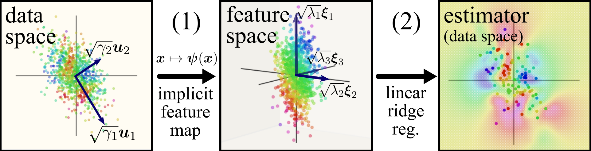
If you’re not yet convinced kernels are the right objects to look at (ie what do these things have to do with practical networks?), you’re right to be sceptical! One of the main drivers behind looking at this simple system and hoping our findings will be useful moving forward is any network’s relation to the Neural Tangent Kernel (NTK), which are an equivalent description of any network if the width of it is taken to infinity, along with some other conditions on the network. While these NTKs can be arbitrarily complex (specifically, those of the transformer and CNNs), the MLP’s neural tangent kernel is rotationally-invariant: in the feature space, distances are calculated solely based off of their difference in angle from the origin. For this reason, we decided to study what the features are of any general rotation-invariant kernel, with a sample schematic of our approach below:
Setup
Rotation invariant kernels can be written mathematically as
where I’ve abused notation a bit. For the data itself , kernel theory says we need to focus on having some fixed distribution from which we get the data from, so we won’t be solving rotation-invariant kernels in totality. Instead, we can note that taking the PCA of a group of images, gives PCA components (which look like blurry images) with marginals being roughly a Gaussian distribution. That means that after taking the PCA of images, any one image can be reconstructed by doing some weighted average of the PCA components, with the weighting being proportional to principal component’s singular value! For theoretical understanding, we thus limit our scope of the problem to solving rotation-invariant kernels on anisotropic Gaussian data:
Component-wise understanding of the kernel
As previously alluded to, there are essentially two steps in kernel regression: the kernel is created, then linear regression is performed. Since linear regression is solved1, we just need to understand the kernel in a way that can be used with the linear regression second step. To do this, previous work (Simon et al., 2021) (other references to be added) have found that an eigendecomposition of the kernel is needed: obtaining the eigenvalues (scales) and eigenvectors (directions) of the kernel is enough to directly predict exactly what the kernel will do, at least in the average case.
where I’ve suggestively wrote the form of our predictor to resemble that of linear regression, giving some sense for the fact that once the eigensystem is found, we just need to apply linear regression thereafter on the features (eigenfunctions) of the data . In the previous work, the eigendecompositon was just solved for numerically without any theoretical backing, so the basis of our paper is to do this analytically!
To give a hint as to how to do this, we can write out the eigensystem equation as follows:
where is the data distribution I mentioned earlier, and is it’s probability distribution. Hopefully as written, it’s more clear that the data will determine the eigensystem of a kernel: any complete basis can be used to describe a kernel, but there is only one that is eigen to the data its being evaluated on.
Kernel-less eigensystem
There’s a neat question one can ask about anisotropic Gaussian data on kernels: for a general kernel, what should we expect the eigenfunctions to look like? How much do we even need to worry about the specifics of any kernel? The answer is, surprisingly, not much… let’s go through it. You can broadly say, “well, the kernel should be able to represent any polynomial of the data,” so we can separate out the features into different levels representing the orders of the polynomials. I’ll give the first one as a freebe as I didn’t motivate it all that much:
- Const mode: = 1, = 1
from there on, we can guess that the data itself (ie a linear function of the data) will be a feature2:
- Linear modes: = , = .
From here on, I hope the pattern has become more obvious, with the next level being…
- Quadratic modes: = , =
- Cubic modes: = , =
Kernel eigensystem
The above picture obviously misses some things, namely the kernel itself. However, our guess is surprisingly close to the real kernel eigensystem!
Eigenvalue fix
To incorporate the kernel, write out the kernel function as a Taylor series expansion:
with this epansion working so long as the points and have roughly the same magnitude, . This turns our rotation-invariant kernel into a dot-product kernel! Being able to express a rotation-invariant kernel as a dot product one is equivalent to having datapoints lie along a hyperellipsoid that “looks spherical enough:” we don’t need the data to exactly lie on the sphere, but if one direction (ie ) holds much more weight than the others, then the data lies more along a line than a sphere, and the expansion breaks. We can start to see where the eigenvalue fix kicks in: let’s take a linear mode to be our eigenfunction we want the eigenvalue of. In the expansion, this will (at least shortly if you’re familiar enough with Guassian distributions) select out only the part of the equation:
where we can see the only fix we need to make to the eigenvalues are to add on an additional factor of to the eigenvalues at level .
In a future update, I will give a small preview of how to obtain these “level coefficients” .
One of the amazing things here is that this is direction-independent so all eigenvalues within a level are affected by the same factor3, and to give a bit of a spoiler, this is the only place the kernel appears! The eigenfunctions need to be fixed in a very simple way:
Eigenfunction fix
The functions = for some general index-selecting object need to be changed so that they’re actually eigenfunctions: they must be an orthonormal basis.
To start, will be on average , not , so the first thing to do is to have = .
The second thing to do is to verify these are actually orthogonal to each other: . This will not be true when there are repeated indices, isn’t orthogonal to , at least when the data is Gaussian-distributed! To get around this, we can simply subtract off whatever the overlapping component is, so . If we continue this pattern (the linear and cubic modes overlap, quadratic and quartic, etc.) then we get the Hermite polynomials.
The Hermite Eigenstructure Ansatz
We can now state the main takeaway of our paper:
Take any rotation-invariant kernel with high-dimensional Gaussian data. The eigensystem of this kernel will be approximately the same as if the eigenvalues and eigenfunctions were given by,
where , , and are the (probabilist’s) Hermite polynomials. We call this the Hermite Eigenstructure Ansatz (HEA), “ansatz” here roughly translated to “approximation” or “guess”.
Checking this numerically, we see a fantastic overlap between the HEA and a real kernel eigensystem:
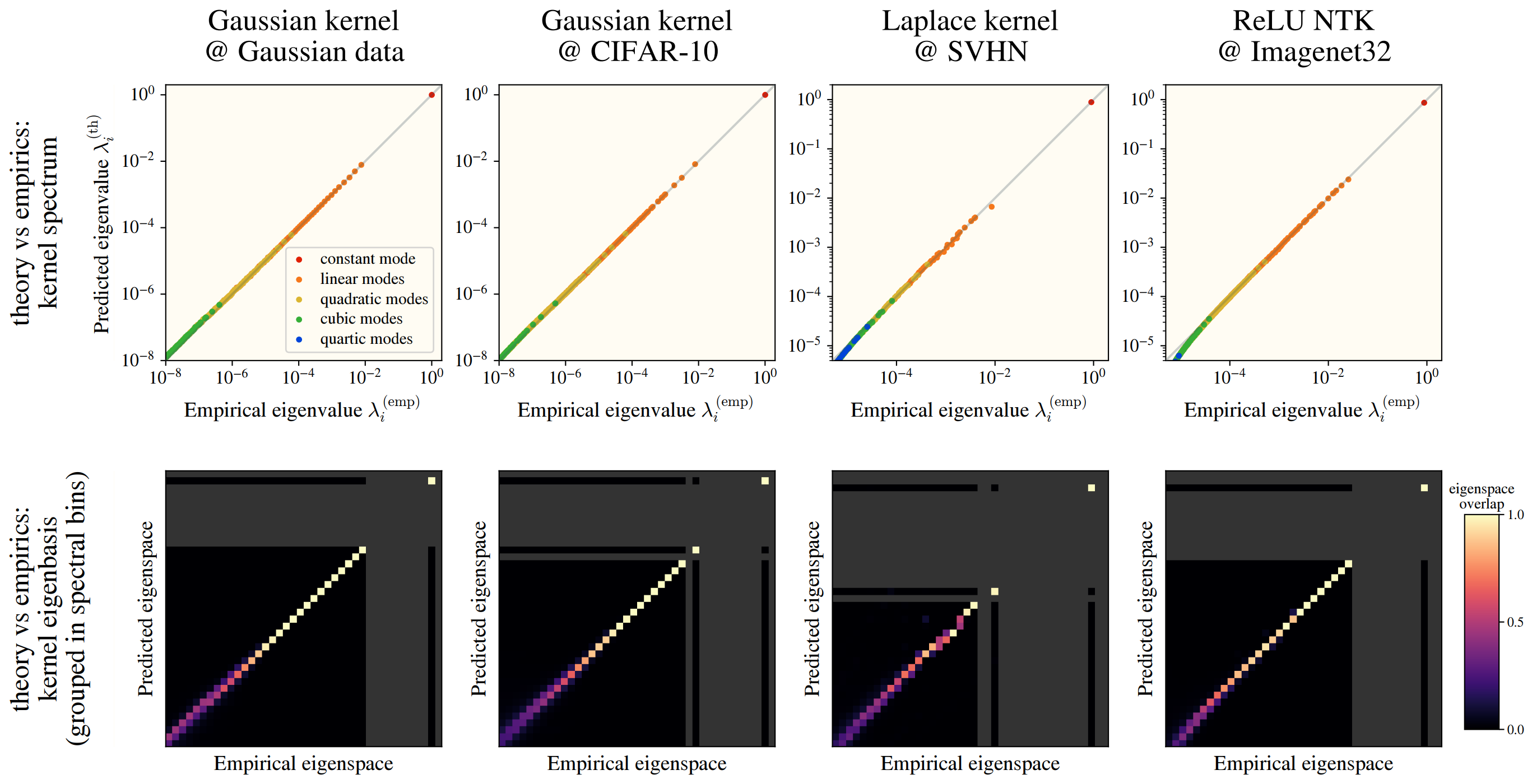
This works among numerous kernels and on real datasets: CIFAR10, SVHN, and ImageNet! In the images, we see how well the -th eigenvalues are approximated by the HEA (top), and the similarity between the HEA-predicted and real eigenvectors (bottom), where we have binned eigenvectors into an “eigenspace” for visual clarity.
The HEA is a guess
Of course, we can’t prove exactly how anything (other than maybe linear regression) performs on real data—there’s a reason we call this the Hermite Eigenstructure Ansatz and not the Hermite Eigenstructure Equivalence. The HEA starts to break down once we get further from the nice land of theory, with 3 key points being required on the data and the kernels: the data lies on something like a hypersphere, the level coefficients decay quickly enough, and the data is We can exactly prove that this Hermite eigensystem is the true eigensystem if we “inverse” these conditions. In slightly more detail,
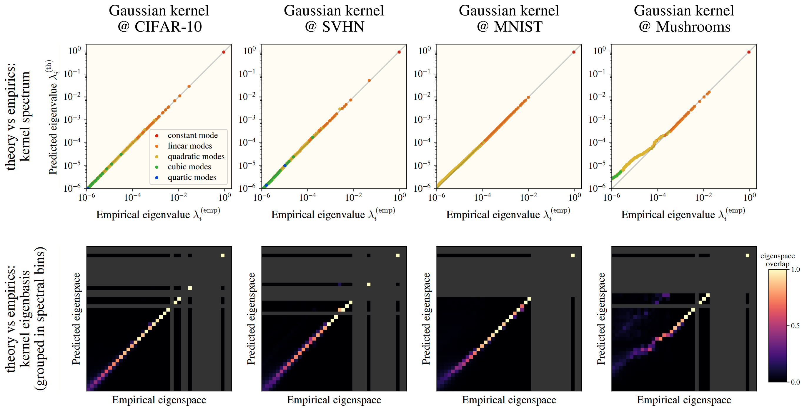
- (High data dimension) If the data is inherently low dimensional, or if a few directions contribute the most to the data’s variance, then the HEA starts breaking down. If there are preferred directions, then the prefactors wouldn’t just depend on the level, and there’s no guarantees the eigenfunctions will be our simple hermites. Certain datasets (namely categorical, see “Mushrooms”) have a few preferred directions, with the exact eigenstructure differences shown below.
- (Fast level coefficient decay) If the level coefficients are “close” to each other, then we get a strange effect: to recover our eigenfunctions as Hermites, we made orthogonal to . That, however, was under the assumption that the eigenvalue corresponding with the degree polynomial was much larger than the polynomial; when this breaks, we end up with a bit of “mutual-orthonormalization” where both the degree and terms interact and try to orthonormalize against the other. In practice, we can sometimes fix this problem by just making the kernel wider; otherwise, the dataset is simply not good for our kernel and HEA.
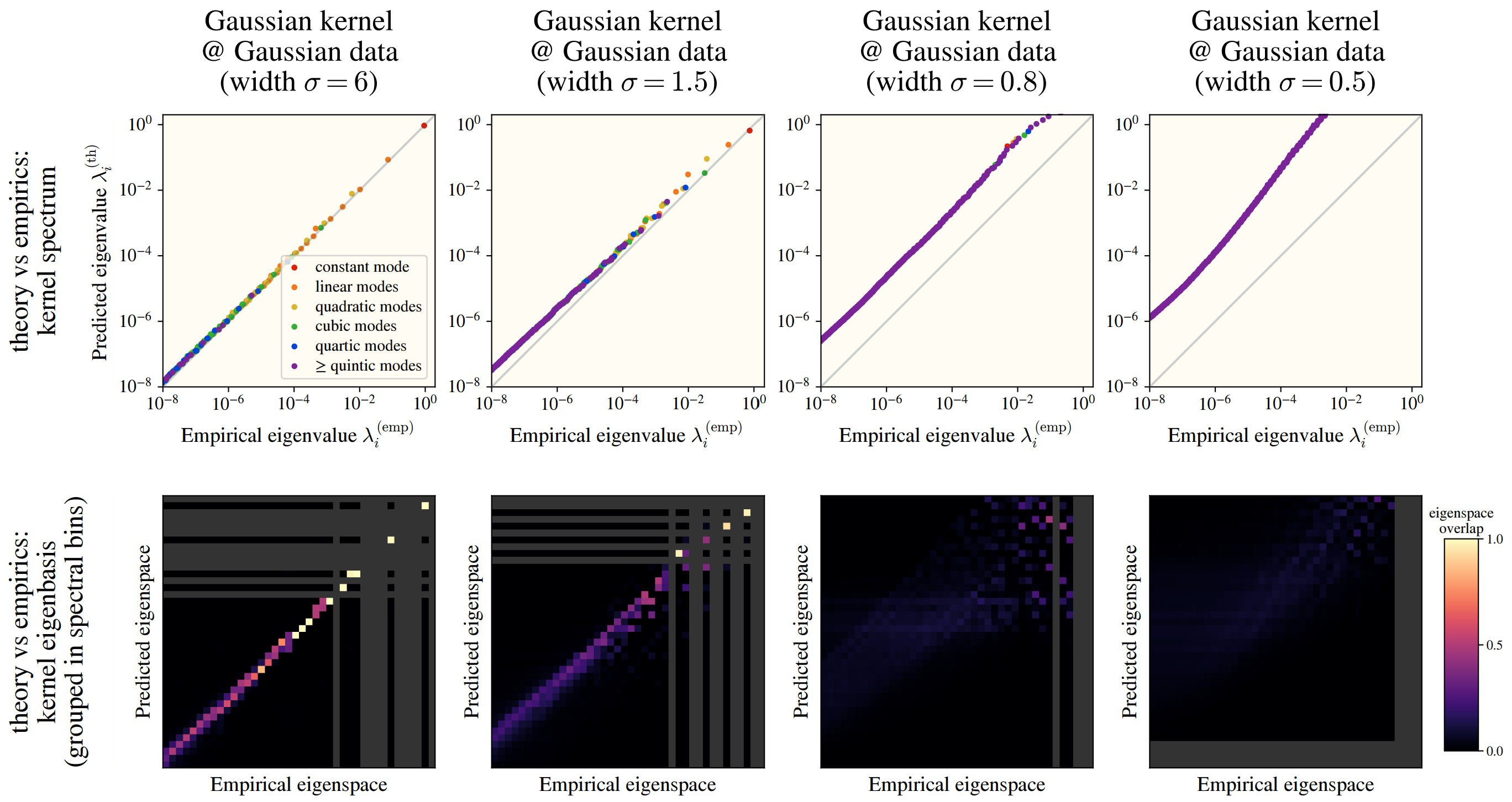
Above, we see that changing the Gaussian kernel’s width can drastically affect how well the HEA works.

Whereas changing the dataset size itself barely changes anything!
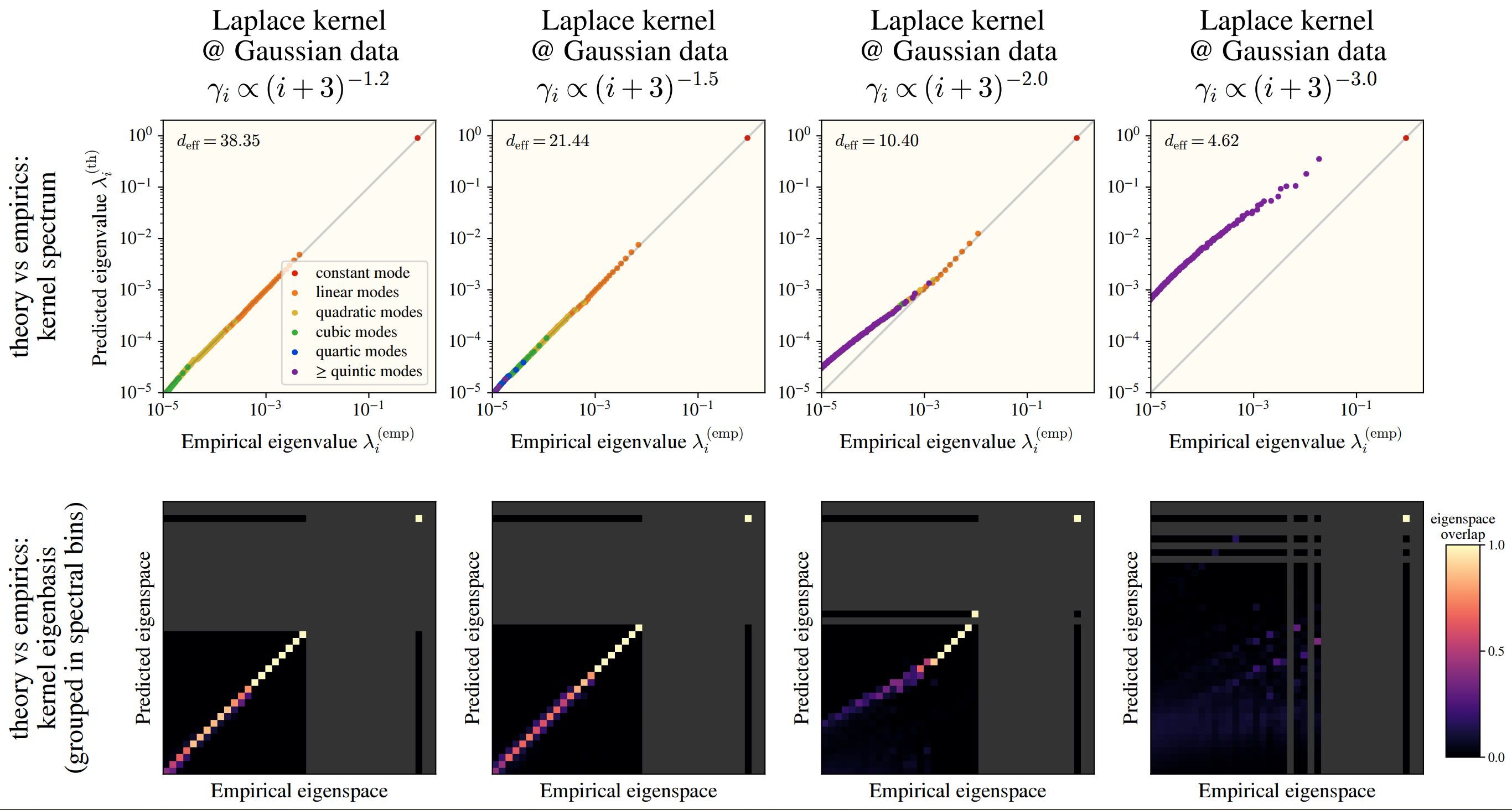
Although this is not true for all kernels! If we take the Gaussian (or ReLU NTK), then the data is far more important!
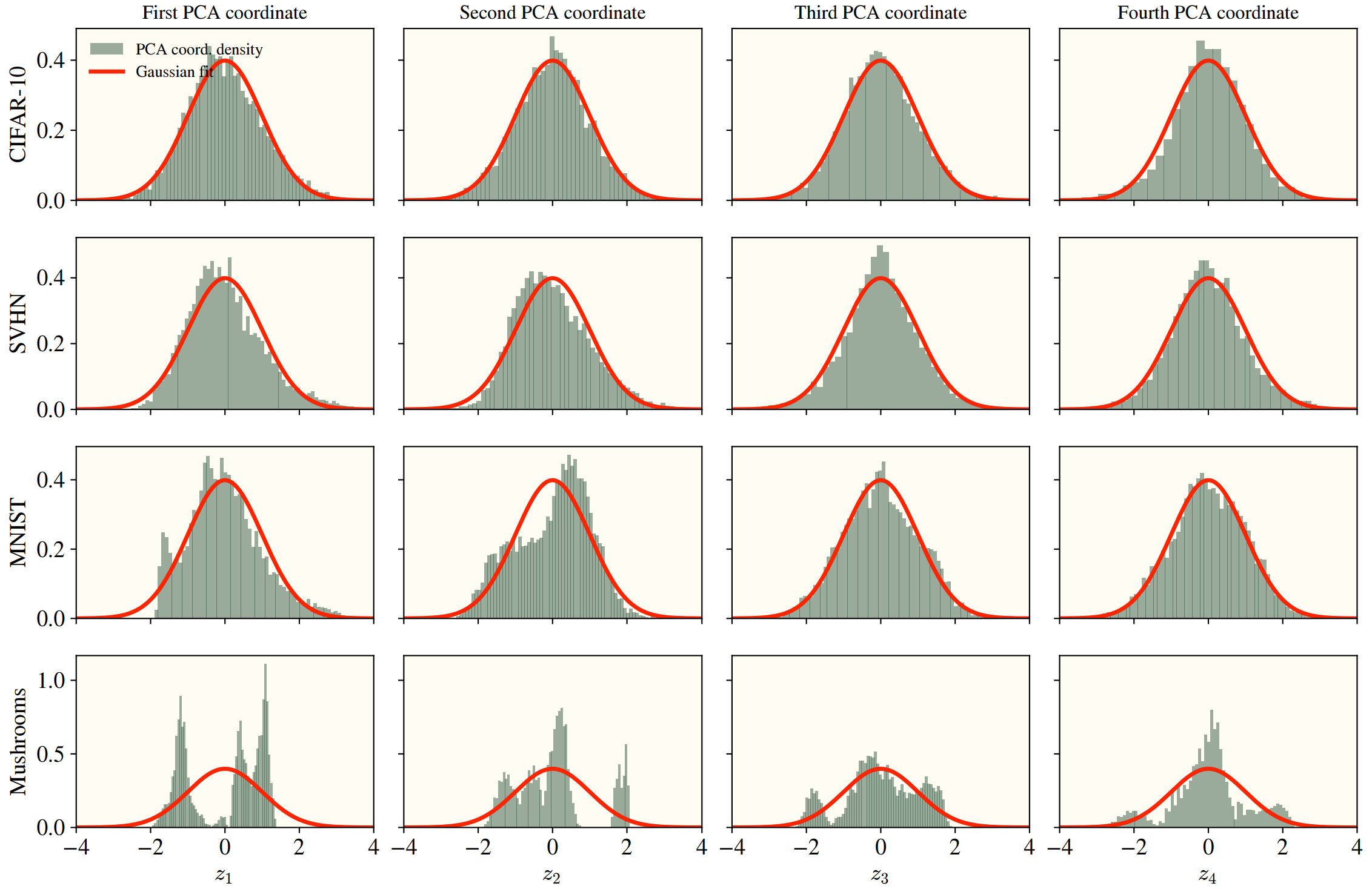
- (Gaussian data) As stated earlier, we need Gaussian data with known covariances—this clearly isn’t true in real settings, so how far does it go if the data isn’t Gaussian? The HEA actually works quite well, unless the PCA components are heavily dependent4 or the marginals are far from being approximated by Gaussian. Independence is hard to visualize, but below I’ve given examples of data that’s far from Gaussian.
HEA to predict learning curves
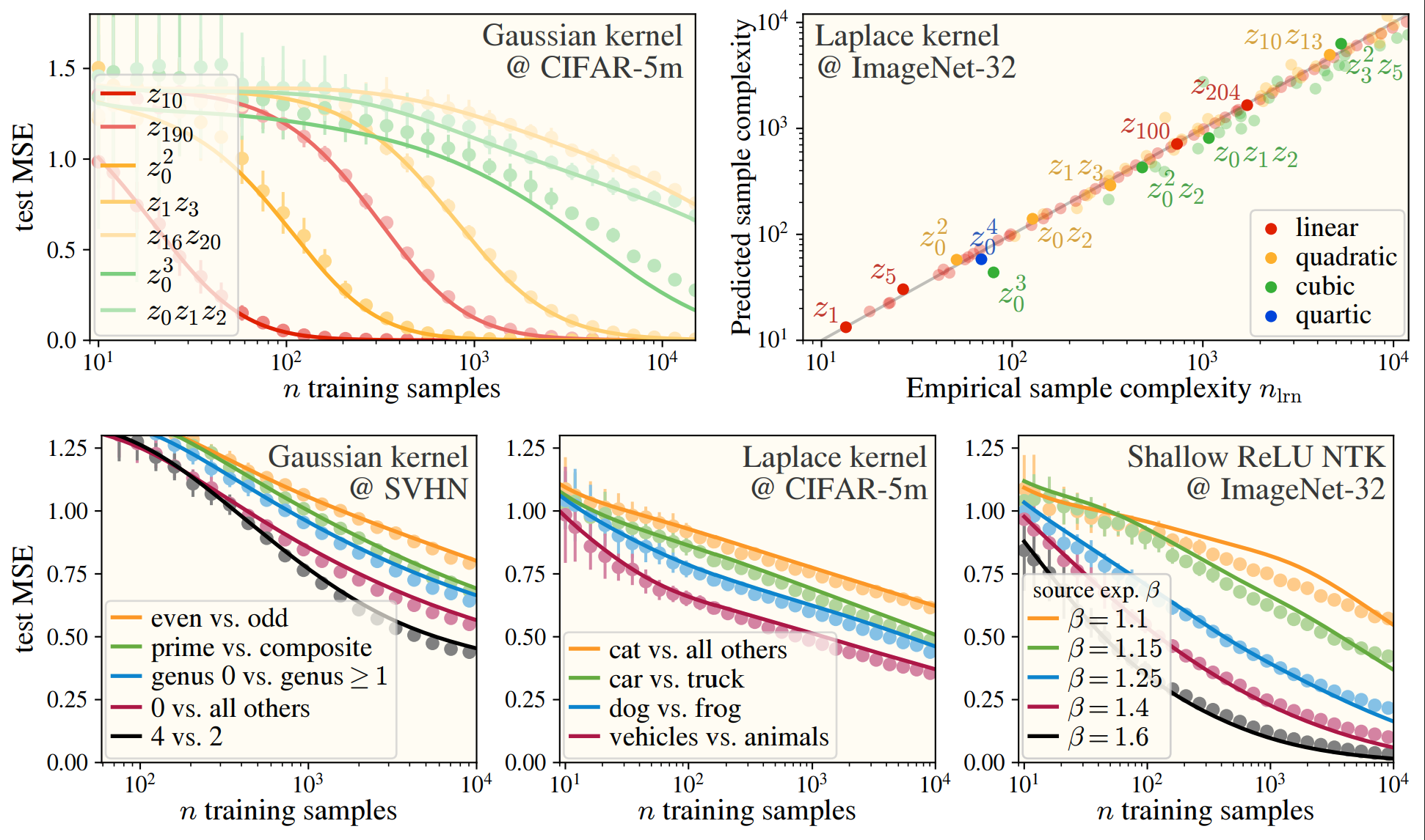
Now we can get to the real takeaway: as we can predict the eigenstructure of the data, we can take our favorite kernel learning curve theory paper (ie (Simon et al., 2021)), and directly predict what the test error, train error, error of specific components, etc. is, or how many samples we need to get below a certain error!
While I’d recommend reading any one of the kernel learning curve theory papers to get a better idea of what’s going on under the hood, I’ll highlight one thing here: the kernel learns the top eigenfunctions when presented with samples. Combined with the HEA, we can get a striking observation, if > , then the sixth-order function corresponding with will be learned before the linear function !
The HEA moving forward
Let’s step back for a little bit. Why should the HEA be at all useful moving forward?
My response: I’ve checked how fast feature-learning networks learn each term in the polynomial expansion of data, and found that the HEA eigenvalues are incredibly predictive of how long it takes a network to learn its corresponding term:
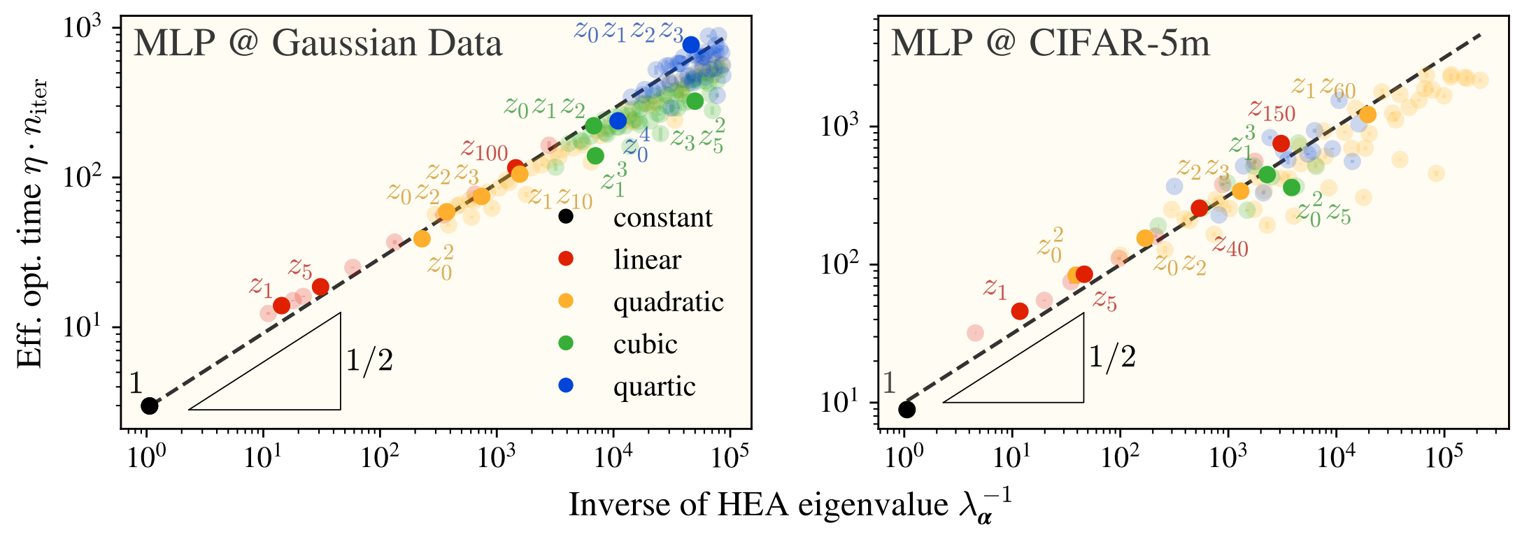
where we’re currently working on understanding where the factor comes from.
Afterword
From here, we’re taking a detour away from kernels and putting a much heavier focus on feature-learning MLPs. If you have questions or comments about any of the content on this page, please feel free to reach out to me! Thanks for reading!
References
Footnotes
-
Solved is a word that holds quite a bit of baggage; luckily, I haven’t found anyone who said linear regression can’t be understood in some principled way. ↩
-
We usually like to have such that the constant mode comes first, but nothing really breaks if this is not true. ↩
-
This is in most part due to the kernel being rotation-invariant. For kernels that are not rotation-invariant, we’d start to see direction-dependent s. ↩
-
PCA is inherently an algorithm that creates dependent components, although some datasets have components that are much more dependent than others. As an example, independent-coordinate isotropic data will be highly dependent under PCA, whereas independent-coordinate highly anisotropic data will have PCA extract the highest anisotropy directions in a much more coordinate-independent manner. ↩